Formatting cells in Excel for a Weapons Mastery Data Tracker

 

For Training Tuesday, we are continuing our series on how to create range reports you can use to identify trends in your marksmanship program using Microsoft Excel. The benefit to this is, it can show trends over time for an organization. All it takes is learning how to manipulate Excel. Today, we will specifically be addressing how to conditionally format cells so you can see trends in large amounts of data, and how to isolate what values can be put into a cell by creating data validation lists.

Conditional formatting of cells in excel allows us to see at a glance what the trends are for an organization. The beautiful thing about doing this is, once the format is set, the cells will adjust when the data changes. So instead of having to go in and color code a bunch of individual cells, I have Excel do the tedious work for me.

So for example; with conditional formatting, I can set up the cells so that when a certain number range is reached, it changes a certain color. Picture 2 illustrates this for us. The cells are formatted so that a score between a 1 and 22 show up red.  23 and a 27 (the minimum to qualify under the draft Integrated Weapons Training Strategy) is orange, Cells between a 28 and 32 show up yellow(Marksman under the draft Integrated Weapons Training Strategy), Cells between a 32 and 35 show up green (sharpshooter under the draft Integrated Weapons Training Strategy), and cells with a value between 36 and 40 show up blue (expert).

 

 

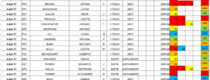
Looking at this section of the document, I can see that over half have qualified first time this is important to pay attention to, as there is only one attempt to qualify in the new Draft Integrated Weapons Training Strategy.

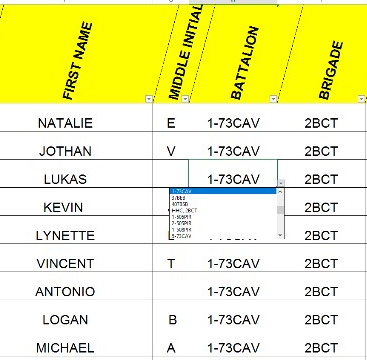
Data validation lists allow you to set up a drop-down selection in a row of cells. Where this is useful is all you have to do is type in the first few characters of the item, and it will come right up to populate the cell. This saves you time when having to input large amounts of data. It also ensures that the appropriate information is input, as it does not allow any deviation from that validation list for the selected range in that row.

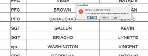
Picture three illustrates this for us. I tried inputting spx instead of SPC in cell D903, and the spreadsheet gives me a warning saying ‘the data you entered is not valid. A user has restricted the values that can be entered into this cell.’ This Ensures that all that gets input is the appropriate rank type. You need this, as when we start discussing pivot tables, if the data is not input the same, you will have three different types of specialist or units populating your tables, counting each as separate categories.

 

 

 

So to sum up, the conditional formatting tool in excel can be used to help identify trends by allowing the data to be looked at in new ways. Once the formatting is established, it requires no additional work on the part of the person inputting the data. The cells automatically adjust as the data changes. Data validation lists allow for a pre-set amount of data to be input into the cells. This makes it more rapid to input and ensures that the data is all the same format. Next week, we will continue our discussion on Excel as we discuss how to do formulas, and what formula types are needed.

 

#weaponsmastery #excelisyourfriend